Gráficos com ggplot2

Soluções

Pacotes necessários

Para fazer estes exercícios, acione os pacotes a seguir:

library(tidyverse)
library(gapminder)
library(ggthemes)

Bancos de dados

starwars

glimpse(starwars)

Rows: 87
Columns: 14
$ name       <chr> "Luke Skywalker", "C-3PO", "R2-D2", "Darth Vader", "Leia Or…
$ height     <int> 172, 167, 96, 202, 150, 178, 165, 97, 183, 182, 188, 180, 2…
$ mass       <dbl> 77.0, 75.0, 32.0, 136.0, 49.0, 120.0, 75.0, 32.0, 84.0, 77.…
$ hair_color <chr> "blond", NA, NA, "none", "brown", "brown, grey", "brown", N…
$ skin_color <chr> "fair", "gold", "white, blue", "white", "light", "light", "…
$ eye_color  <chr> "blue", "yellow", "red", "yellow", "brown", "blue", "blue",…
$ birth_year <dbl> 19.0, 112.0, 33.0, 41.9, 19.0, 52.0, 47.0, NA, 24.0, 57.0, …
$ sex        <chr> "male", "none", "none", "male", "female", "male", "female",…
$ gender     <chr> "masculine", "masculine", "masculine", "masculine", "femini…
$ homeworld  <chr> "Tatooine", "Tatooine", "Naboo", "Tatooine", "Alderaan", "T…
$ species    <chr> "Human", "Droid", "Droid", "Human", "Human", "Human", "Huma…
$ films      <list> <"A New Hope", "The Empire Strikes Back", "Return of the J…
$ vehicles   <list> <"Snowspeeder", "Imperial Speeder Bike">, <>, <>, <>, "Imp…
$ starships  <list> <"X-wing", "Imperial shuttle">, <>, <>, "TIE Advanced x1",…

gapminder

glimpse(gapminder)

Rows: 1,704
Columns: 6
$ country   <fct> "Afghanistan", "Afghanistan", "Afghanistan", "Afghanistan", …
$ continent <fct> Asia, Asia, Asia, Asia, Asia, Asia, Asia, Asia, Asia, Asia, …
$ year      <int> 1952, 1957, 1962, 1967, 1972, 1977, 1982, 1987, 1992, 1997, …
$ lifeExp   <dbl> 28.801, 30.332, 31.997, 34.020, 36.088, 38.438, 39.854, 40.8…
$ pop       <int> 8425333, 9240934, 10267083, 11537966, 13079460, 14880372, 12…
$ gdpPercap <dbl> 779.4453, 820.8530, 853.1007, 836.1971, 739.9811, 786.1134, …

Nota

Do exercício 1 até o exercício 8, você vai utilizar o banco de dados starwars

Exercício 1

starwars |>
  drop_na(sex) |> 
  ggplot(aes(sex)) +
  geom_bar()

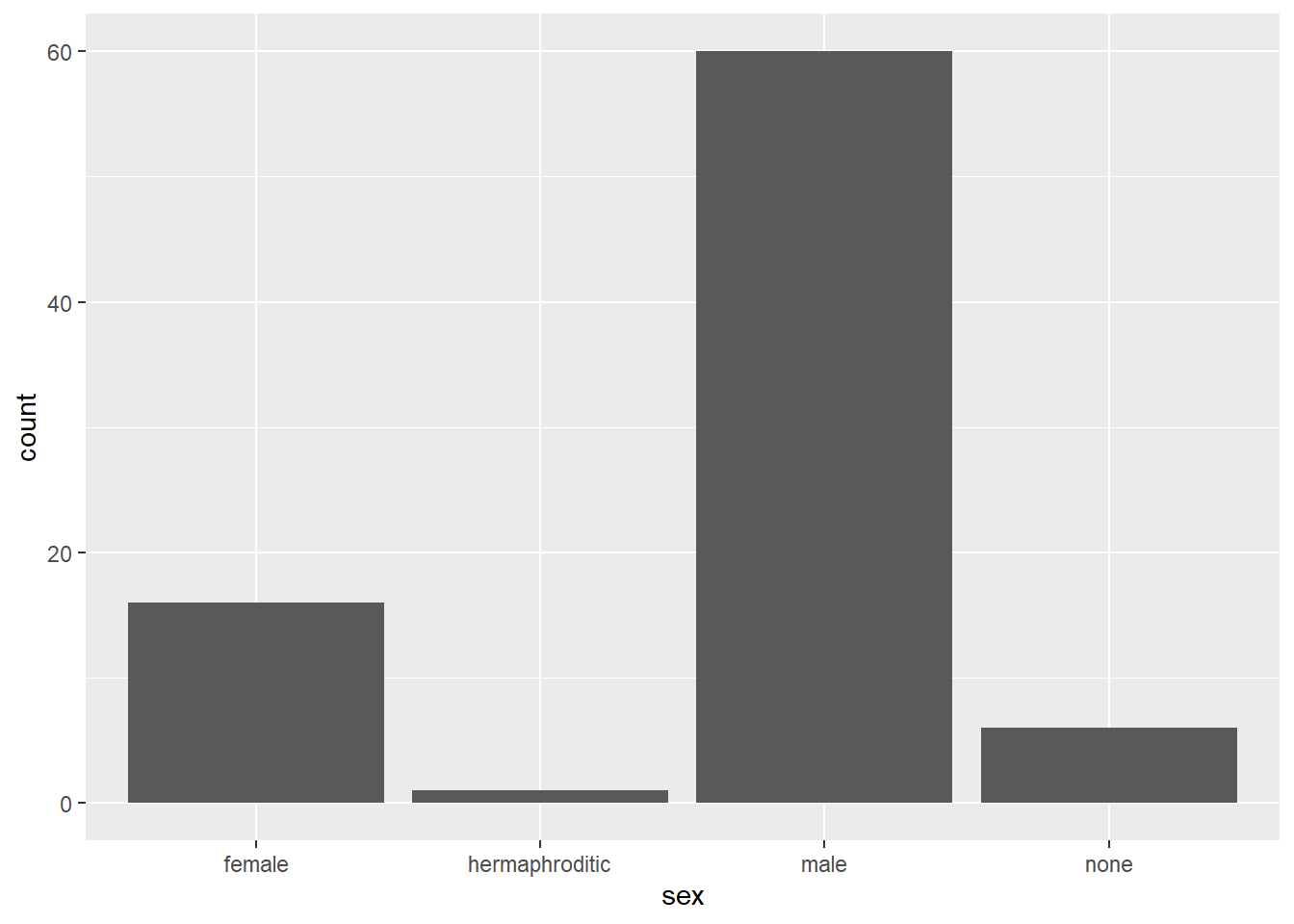
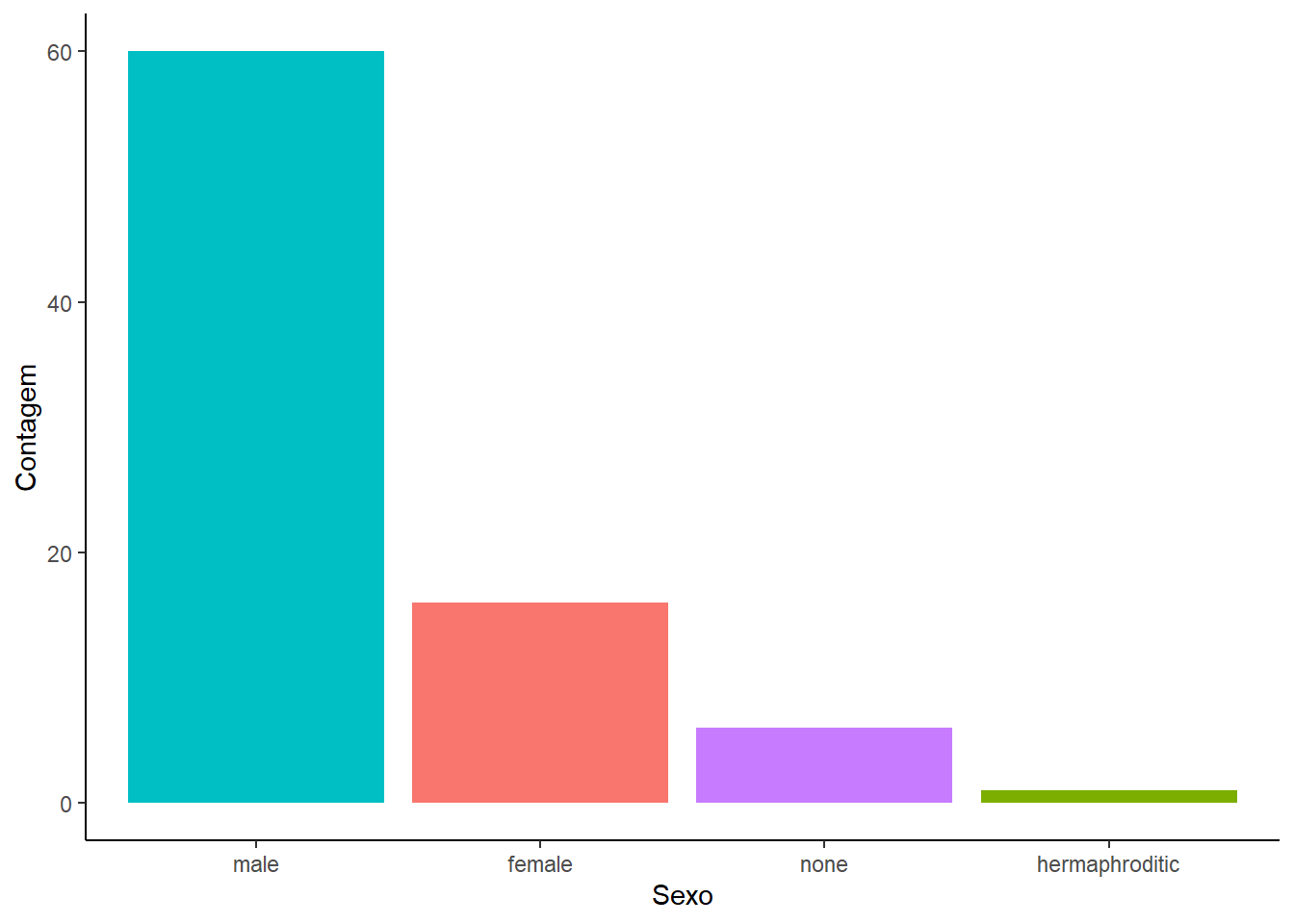
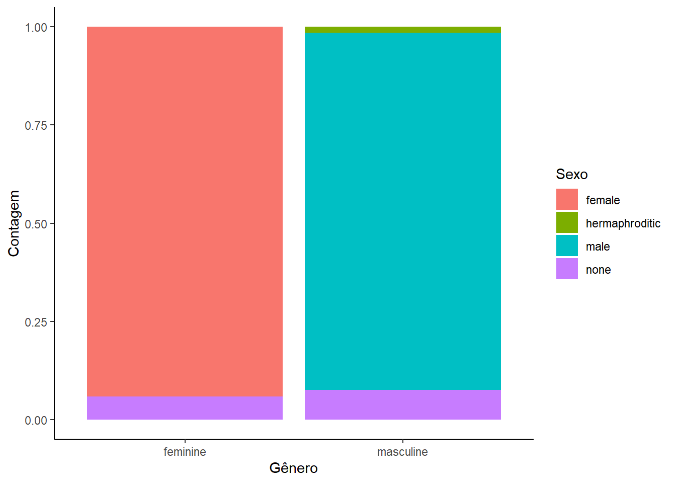
Exercício 2

starwars |>
  drop_na(sex) |> 
  ggplot(aes(fct_infreq(sex), fill = sex)) +
  geom_bar() +
  labs(
    x = "Sexo",
    y = "Contagem"
    ) +
  theme_classic() +
  theme(
    legend.position = "none"
    )

Exercício 3

starwars |> 
  drop_na(sex,gender) |> 
  ggplot(aes(gender, fill = sex)) +
  geom_bar(
    position = "fill"
    )

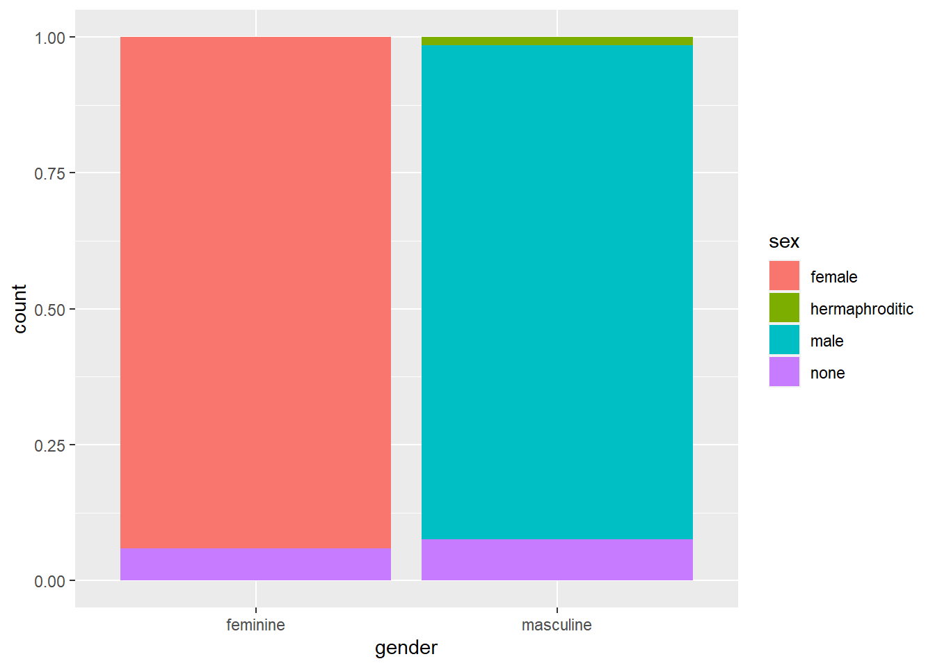
Exercício 4

starwars |> 
  drop_na(sex,gender) |> 
  ggplot(aes(gender, fill = sex)) +
  geom_bar(
    position = "fill"
    ) +
  labs(
    x = "Gênero",
    y = "Contagem",
    fill = "Sexo"
  ) +
  theme_classic()

Exercício 5

starwars |> 
  ggplot(aes(height)) +
  geom_histogram(bins = 18)

Warning: Removed 6 rows containing non-finite values (`stat_bin()`).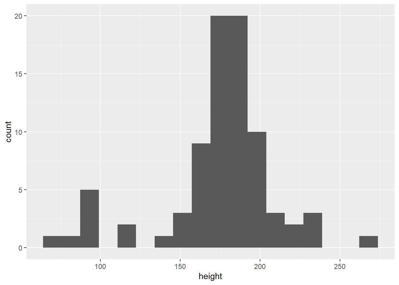

Exercício 6

starwars |> 
  ggplot(aes(height)) +
  geom_histogram(
    bins = 18,
    color = "black", 
    fill = "gray"
    ) +
  labs(
    x = "Altura (cm)",
    y = NULL
  ) + 
  theme_light() 

Warning: Removed 6 rows containing non-finite values (`stat_bin()`).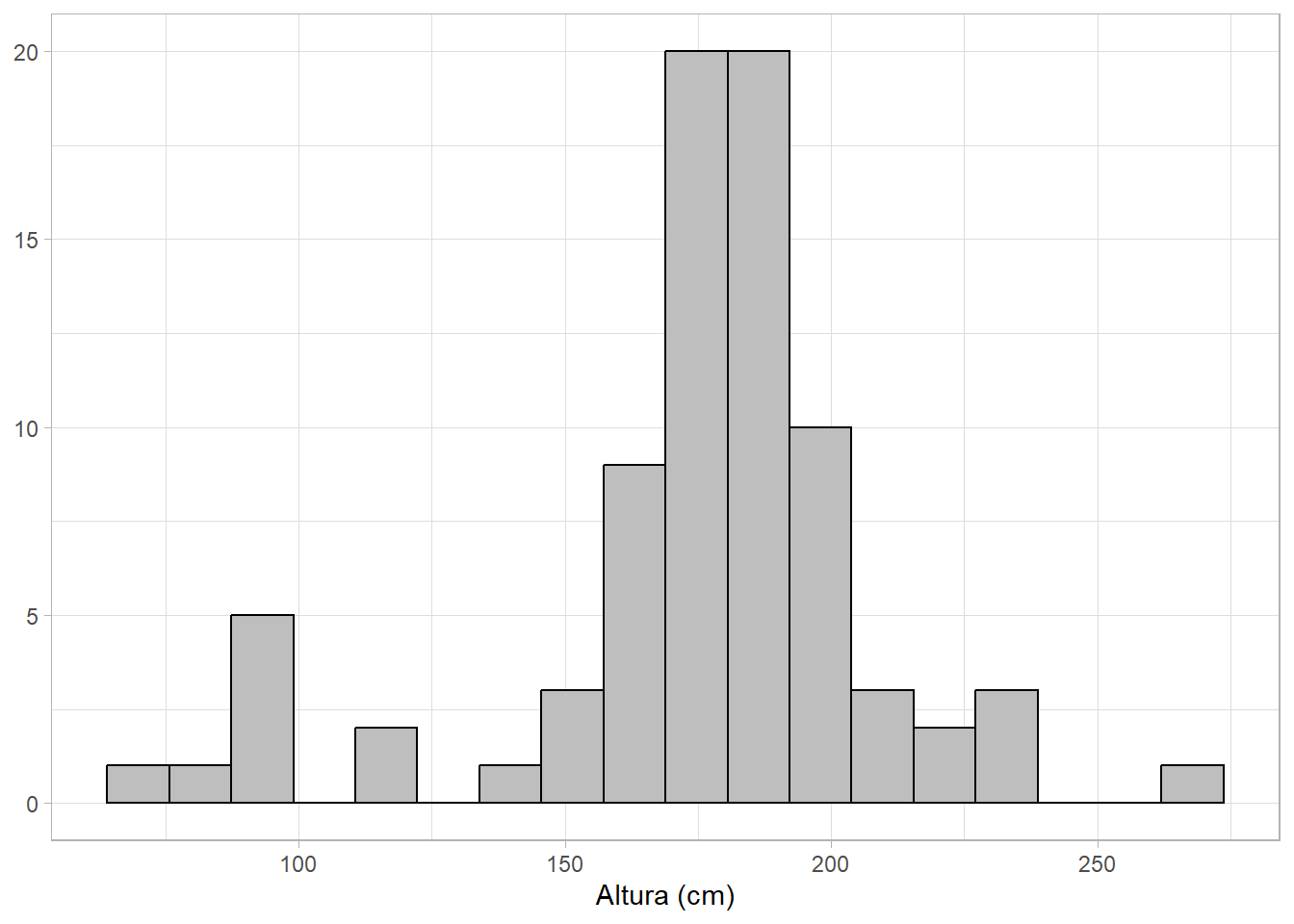

Exercício 7

starwars |>
  drop_na(species, height) |>  
  mutate(
    species = fct_lump_n(species, n = 3)
  ) |> 
  ggplot(aes(species, height)) +
  geom_boxplot()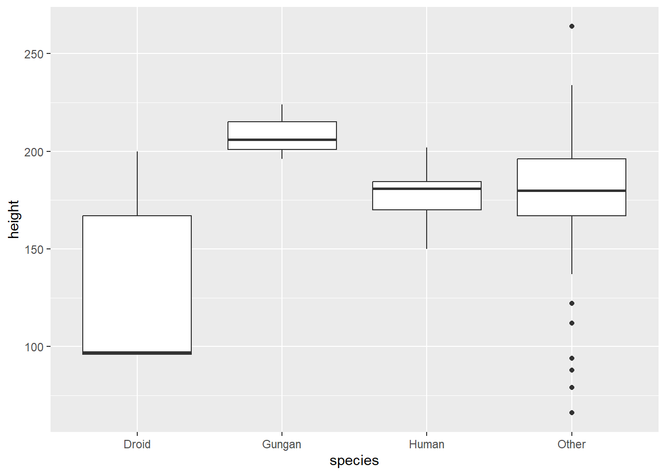

Exercício 8

starwars |> 
  drop_na(species, height) |> 
  mutate(
    species = fct_lump_n(species, 3)
  ) |> 
  ggplot(aes(fct_reorder(species, height),height)) +
  geom_boxplot() + 
  geom_jitter(
    color = "red",
    alpha = 0.2
    ) +
  labs(
    x = "Espécies",
    y = "Altura"
  ) +
  theme_light()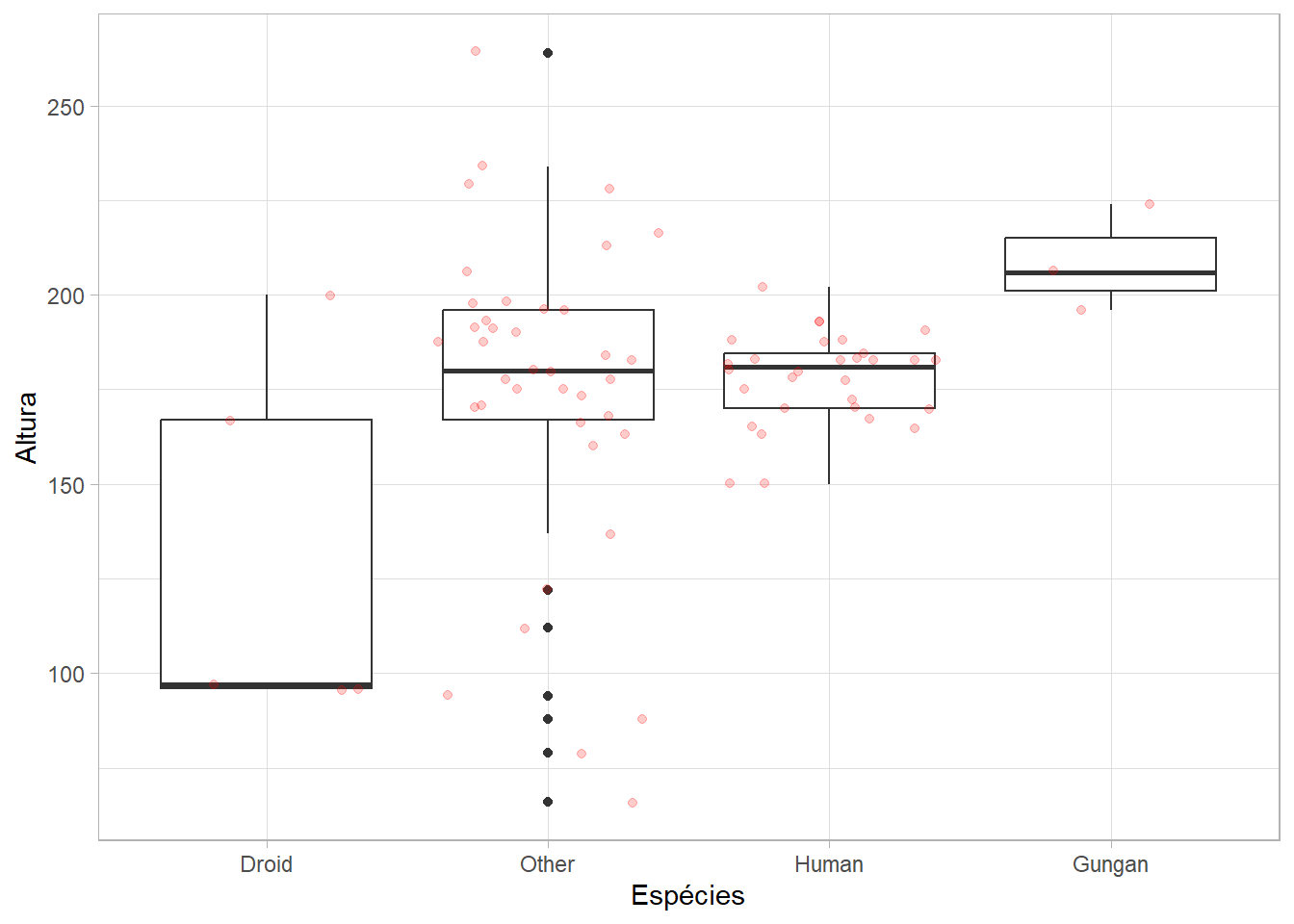

Nota

A partir do exercício 9, você vai utilizar o banco de dados gapminder.

Exercício 9

gapminder |>
  filter(year == 2007) |> 
  ggplot(aes(gdpPercap, lifeExp)) +
  geom_point()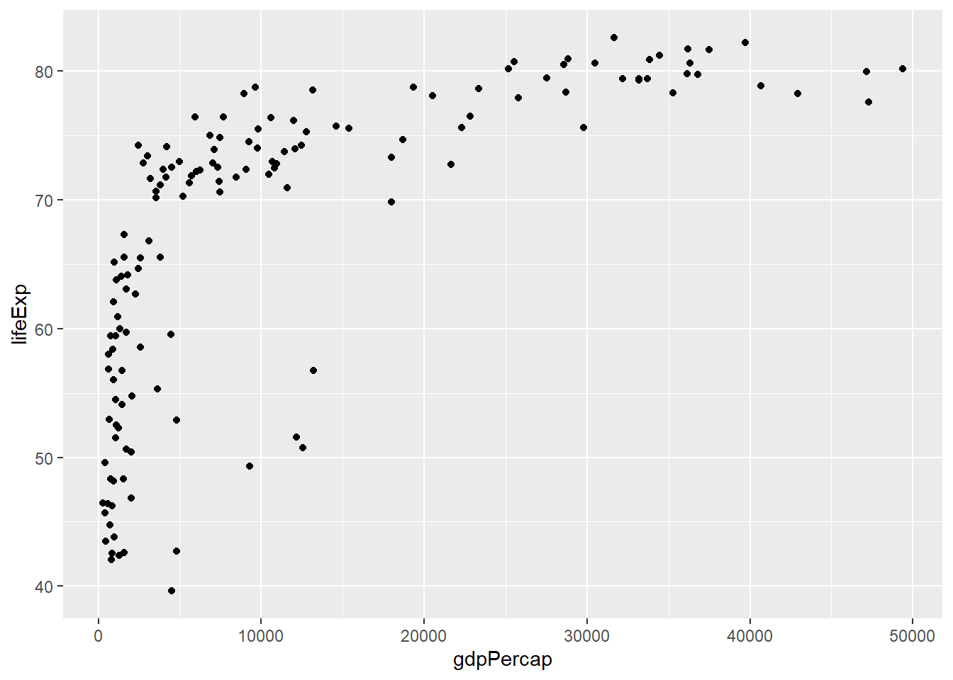

Exercício 10

gapminder |>
  filter(year == 2007) |> 
  ggplot(aes(log(gdpPercap), lifeExp)) +
  geom_point(aes(color = continent,
                 shape = continent)) +
  labs(
    x = "PIB per capita",
    y = "Expectativa de vida",
    color = "Continente",
    shape = "Continente",
    title = "Relação entre expectativa de vida e PIB per capita:",
    subtitle = "Distribuição por continente em 2007"
  ) +
  scale_color_colorblind() +
  theme_classic()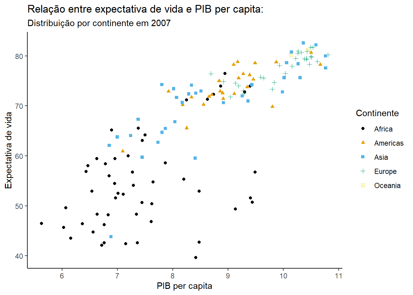

Exercício 11

gapminder |> 
  filter(year == 1952) |> 
  ggplot(aes(log(gdpPercap) , lifeExp, )) +
  geom_point(aes(color = continent, shape = continent)) +
  scale_color_colorblind() +
  facet_wrap(~ continent)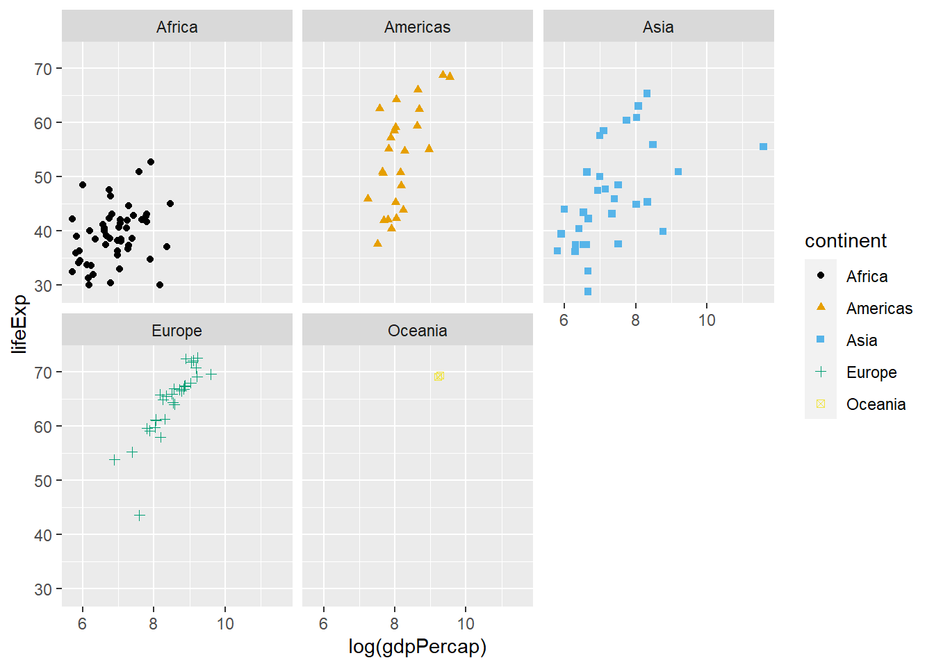

Exercício 12

gapminder |> 
  filter(year == 1952) |> 
  ggplot(aes(log(gdpPercap), lifeExp)) +
  geom_point(aes(color = continent, shape = continent)) +
  facet_wrap(~ continent) +
  labs(
    x = "PIB per capita",
    y = "Expectativa de Vida",
    title = "Relação entre PIB per capita e expectativa de vida por continente",
    subtitle = "1952"
  ) +
  scale_color_colorblind() +
  theme_clean() +
  theme(legend.position = "none")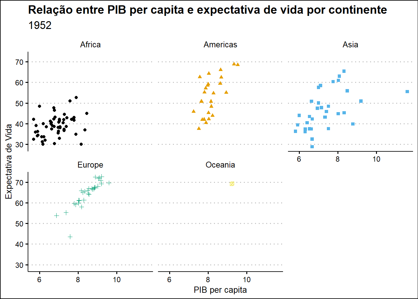

Exercício 13

gapminder |> 
  group_by(continent, year) |> 
  summarise(lifeExp = mean(lifeExp)) |> 
  ggplot(aes(year, lifeExp, color = continent)) +
  geom_line() +
  geom_point()

`summarise()` has grouped output by 'continent'. You can override using the
`.groups` argument.

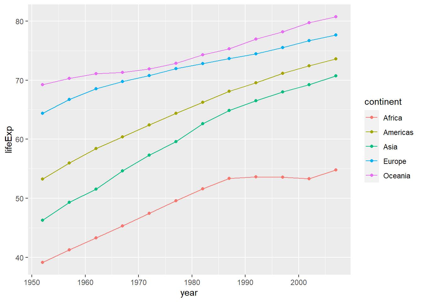
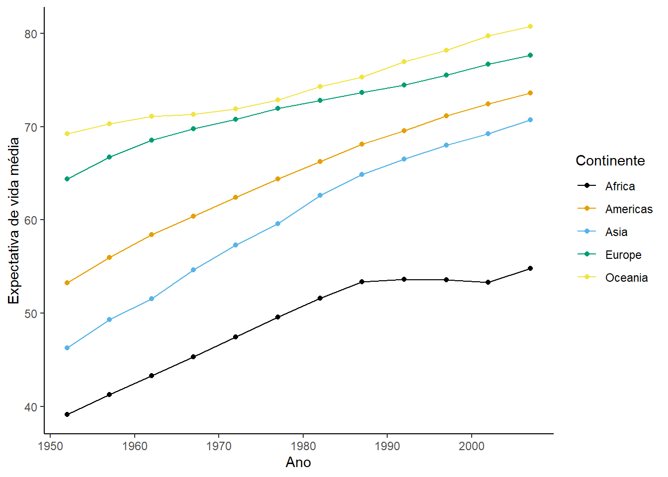
Exercício 14

gapminder |> 
  group_by(continent, year) |> 
  summarise(lifeExp = mean(lifeExp)) |> 
  ggplot(aes(year, lifeExp, color = continent)) +
  geom_line() +
  geom_point() +
  labs(
    x = "Ano",
    y = "Expectativa de vida média",
    color = "Continente"
  ) +
  scale_color_colorblind() +
  theme_classic()

`summarise()` has grouped output by 'continent'. You can override using the
`.groups` argument.