Introdução ao R para análise de dados em Psicologia

Francisco Pablo Huascar Aragão Pinheiro

Quem sou eu

Psicólogo (UFC)
Mestre em Psicologia (UFC)
Doutor em educação (UFC)
Professor do campus Sobral da UFC
Recentemente, um entusiasta do R

Regressão

Statistical Inference via Data Science: A ModernDive into R and the Tidyverse

Livro base para o aprendizado sobre regressão

Capa do livro R for Data Science. Uma coruja se destaca na ilustração

Statistical Inference via Data Science: A ModernDive into R and the Tidyverse

Neste link você pode acessar o livro:

https://moderndive.com/index.html/

Pacotes utilizados

library(tidyverse)
library(tidymodels)

Obtenção do banco de dados

if(!file.exists("./data")){dir.create("./data")}

df <- read_csv("https://tinyurl.com/contextosm")

Uma olhada no banco de dados

glimpse(df)

Rows: 1,000
Columns: 98
$ a1                             <dbl> 1, 1, 1, 1, 2, 2, 2, 1, 1, 3, 2, 1, 1, …
$ a2                             <dbl> 1, 1, 1, 1, 1, 1, 2, 1, 1, 3, 2, 1, 1, …
$ a3                             <dbl> 1, 1, 1, 1, 3, 1, 2, 1, 1, 2, 2, 1, 1, …
$ a4                             <dbl> 1, 1, 2, 1, 2, 1, 2, 1, 1, 3, 3, 1, 1, …
$ a5                             <dbl> 1, 1, 1, 1, 1, 1, 2, 1, 1, 2, 2, 1, 1, …
$ a6                             <dbl> 1, 1, 1, 1, 1, 1, 2, 1, 1, 2, 2, 1, 1, …
$ a7                             <dbl> 1, 1, 1, 1, 2, 1, 3, 1, 1, 2, 2, 1, 1, …
$ d1                             <dbl> 1, 1, 1, 1, 1, 2, 1, 1, 1, 3, 2, 1, 1, …
$ d2                             <dbl> 1, 1, 1, 1, 1, 2, 1, 1, 1, 3, 2, 1, 1, …
$ d3                             <dbl> 1, 1, 1, 1, 2, 2, 2, 1, 1, 3, 2, 1, 1, …
$ d4                             <dbl> 1, 1, 1, 1, 2, 2, 1, 1, 1, 2, 2, 1, 1, …
$ d5                             <dbl> 1, 1, 1, 1, 1, 1, 1, 1, 1, 2, 2, 1, 1, …
$ d6                             <dbl> 1, 1, 1, 1, 1, 2, 1, 1, 1, 2, 2, 1, 1, …
$ d7                             <dbl> 1, 1, 1, 1, 2, 1, 1, 1, 1, 2, 2, 1, 1, …
$ e1                             <dbl> 1, 1, 1, 1, 2, 2, 2, 1, 1, 3, 2, 1, 1, …
$ e2                             <dbl> 1, 1, 1, 1, 1, 2, 1, 1, 1, 3, 2, 1, 1, …
$ e3                             <dbl> 1, 1, 1, 1, 2, 2, 2, 1, 1, 2, 2, 1, 1, …
$ e4                             <dbl> 1, 1, 2, 1, 3, 2, 2, 1, 1, 3, 2, 1, 1, …
$ e5                             <dbl> 1, 1, 2, 1, 3, 2, 2, 1, 1, 2, 2, 1, 2, …
$ e6                             <dbl> 1, 1, 1, 1, 1, 2, 1, 1, 1, 2, 2, 1, 1, …
$ e7                             <dbl> 1, 1, 1, 1, 2, 2, 3, 1, 1, 2, 2, 1, 1, …
$ ct1                            <dbl> 1, 1, 3, 3, 4, 4, 4, 3, 4, 3, 3, 1, 3, …
$ ct2                            <dbl> 1, 1, 3, 1, 1, 4, 3, 2, 3, 4, 1, 1, 4, …
$ ct3                            <dbl> 1, 1, 2, 1, 4, 4, 3, 1, 1, 1, 4, 1, 1, …
$ ct4                            <dbl> 1, 1, 3, 3, 4, 2, 4, 3, 4, 3, 1, 1, 5, …
$ ct5                            <dbl> 1, 1, 2, 5, 1, 3, 3, 3, 1, 4, 4, 1, 3, …
$ ct6                            <dbl> 1, 1, 2, 1, 1, 2, 3, 2, 1, 2, 3, 1, 1, …
$ ct7                            <dbl> 1, 1, 3, 3, 4, 4, 4, 3, 3, 3, 4, 1, 3, …
$ ct8                            <dbl> 1, 1, 3, 3, 3, 4, 4, 3, 3, 1, 2, 4, 2, …
$ ct9                            <dbl> 1, 1, 2, 3, 2, 3, 3, 2, 3, 2, 5, 1, 1, …
$ ct10                           <dbl> 1, 1, 2, 1, 1, 3, 3, 3, 3, 4, 2, 1, 2, …
$ ct11                           <dbl> 1, 1, 2, 5, 1, 2, 3, 2, 1, 4, 3, 2, 3, …
$ ct12                           <dbl> 1, 1, 4, 5, 3, 5, 5, 3, 4, 4, 5, 5, 3, …
$ ct13                           <dbl> 1, 1, 2, 5, 2, 5, 4, 3, 2, 4, 3, 5, 3, …
$ ct14                           <dbl> 1, 1, 3, 3, 2, 5, 4, 3, 3, 4, 5, 4, 4, …
$ ct15                           <dbl> 1, 1, 2, 3, 1, 2, 3, 2, 1, 3, 3, 3, 3, …
$ ct16                           <dbl> 1, 1, 3, 3, 2, 4, 3, 3, 2, 3, 5, 1, 2, …
$ ct17                           <dbl> 1, 1, 3, 3, 2, 3, 3, 2, 1, 1, 5, 5, 2, …
$ ct18                           <dbl> 1, 1, 3, 2, 3, 3, 5, 3, 4, 4, 3, 5, 1, …
$ ct19                           <dbl> 1, 1, 3, 3, 2, 3, 4, 3, 3, 1, 5, 1, 3, …
$ ct20                           <dbl> 1, 1, 3, 3, 3, 3, 4, 3, 2, 1, 5, 2, 3, …
$ ct21                           <dbl> 1, 1, 3, 3, 3, 3, 3, 2, 2, 1, 3, 3, 3, …
$ ct22                           <dbl> 1, 1, 2, 3, 4, 3, 3, 3, 1, 3, 3, 1, 3, …
$ ct23                           <dbl> 1, 1, 3, 1, 3, 3, 4, 3, 3, 2, 5, 1, 3, …
$ ct24                           <dbl> 1, 1, 3, 5, 1, 3, 3, 2, 1, 1, 3, 3, 3, …
$ ct25                           <dbl> 1, 1, 2, 1, 3, 3, 2, 3, 2, 4, 3, 3, 2, …
$ ct26                           <dbl> 1, 1, 3, 3, 4, 3, 4, 3, 2, 4, 5, 3, 1, …
$ ct27                           <dbl> 1, 1, 3, 1, 1, 4, 3, 3, 1, 1, 5, 1, 4, …
$ ct28                           <dbl> 1, 1, 2, 3, 1, 4, 3, 3, 3, 2, 3, 1, 1, …
$ ct29                           <dbl> 1, 1, 2, 1, 2, 3, 3, 3, 3, 3, 3, 3, 1, …
$ ct30                           <dbl> 1, 1, 2, 1, 1, 5, 3, 5, 2, 1, 5, 2, 4, …
$ ct31                           <dbl> 1, 1, 1, 1, 1, 2, 1, 2, 1, 5, 3, 1, 1, …
$ ct32                           <dbl> 1, 1, 2, 1, 1, 2, 2, 1, 1, 1, 3, 2, 2, …
$ ct33                           <dbl> 1, 1, 2, 1, 1, 3, 3, 3, 1, 1, 3, 2, 1, …
$ ct34                           <dbl> 1, 1, 3, 3, 2, 4, 3, 2, 2, 1, 3, 5, 1, …
$ ct35                           <dbl> 1, 1, 3, 1, 1, 2, 2, 4, 1, 5, 3, 2, 1, …
$ ct36                           <dbl> 1, 1, 2, 1, 1, 3, 4, 4, 2, 2, 3, 1, 2, …
$ ct37                           <dbl> 1, 1, 2, 1, 1, 5, 3, 3, 1, 3, 3, 4, 3, …
$ ct38                           <dbl> 1, 1, 2, 3, 2, 3, 4, 3, 3, 5, 5, 2, 2, …
$ ct39                           <dbl> 1, 1, 2, 1, 1, 3, 2, 1, 1, 5, 3, 2, 3, …
$ ct40                           <dbl> 1, 1, 4, 1, 2, 3, 3, 3, 4, 5, 5, 5, 1, …
$ srq1                           <dbl> 0, 0, 0, 0, 0, 1, 1, 0, 0, 1, 1, 0, 1, …
$ srq2                           <dbl> 0, 0, 0, 0, 0, 1, 0, 0, 0, 1, 1, 0, 0, …
$ srq3                           <dbl> 0, 0, 0, 0, 1, 1, 1, 0, 0, 1, 1, 0, 1, …
$ srq4                           <dbl> 0, 0, 0, 0, 0, 1, 1, 0, 1, 1, 1, 0, 0, …
$ srq5                           <dbl> 0, 0, 0, 0, 0, 0, 1, 0, 0, 1, 0, 0, 0, …
$ srq6                           <dbl> 0, 1, 1, 0, 1, 1, 1, 0, 0, 1, 1, 0, 0, …
$ srq7                           <dbl> 0, 0, 0, 0, 1, 1, 0, 0, 0, 1, 1, 0, 0, …
$ srq8                           <dbl> 0, 0, 0, 1, 1, 1, 0, 0, 0, 1, 0, 0, 0, …
$ srq9                           <dbl> 0, 0, 0, 0, 1, 1, 1, 0, 0, 1, 1, 0, 0, …
$ srq10                          <dbl> 0, 0, 0, 0, 0, 1, 1, 0, 0, 1, 1, 0, 0, …
$ srq11                          <dbl> 0, 0, 0, 0, 0, 1, 0, 0, 0, 1, 1, 0, 0, …
$ srq12                          <dbl> 0, 1, 0, 0, 0, 1, 1, 0, 0, 1, 1, 0, 0, …
$ srq13                          <dbl> 0, 0, 0, 0, 1, 1, 0, 0, 0, 1, 0, 0, 0, …
$ srq14                          <dbl> 0, 0, 0, 0, 0, 1, 0, 0, 0, 1, 0, 0, 0, …
$ srq15                          <dbl> 0, 0, 0, 0, 0, 1, 0, 0, 0, 1, 0, 0, 0, …
$ srq16                          <dbl> 0, 0, 0, 0, 0, 0, 0, 0, 0, 1, 0, 0, 0, …
$ srq17                          <dbl> 0, 0, 0, 0, 0, 0, 0, 0, 0, 1, 0, 0, 0, …
$ srq18                          <dbl> 0, 0, 0, 0, 0, 1, 1, 0, 0, 1, 0, 0, 0, …
$ srq19                          <dbl> 0, 0, 0, 0, 1, 1, 1, 0, 0, 1, 1, 0, 0, …
$ srq20                          <dbl> 0, 0, 0, 0, 1, 1, 1, 0, 0, 1, 1, 0, 0, …
$ genero                         <chr> "Feminino", "Feminino", "Feminino", "Fe…
$ idade                          <dbl> 37, 46, 44, 46, 46, 36, 41, 61, 37, 25,…
$ cor_raca                       <chr> "Pardo", "Pardo", "Pardo", "Pardo", "Pa…
$ escolaridade                   <chr> "Especialização", "Especialização", "Es…
$ estado_civil                   <chr> "Casado(a)", "Solteiro(a)", "Divorciado…
$ filhos                         <dbl> 2, 1, 2, 2, 0, 0, 1, 2, 1, 0, 2, 0, 0, …
$ renda_familiar_mensal          <dbl> 4000, 4000, 4000, 3500, 6600, 4000, 300…
$ dependentes_da_renda_familar   <dbl> 4, 3, 2, 3, 3, 5, 2, 1, 3, 7, 3, 1, 2, …
$ renda_pos_pandemia             <chr> "Aumentou", "Diminuiu", "Ficou estável"…
$ estado                         <chr> "Tocantins", "Ceará", "Pernambuco", "Ce…
$ regiao                         <chr> "Norte", "Nordeste", "Nordeste", "Norde…
$ grupo_de_risco                 <chr> "Não", "Sim", "Não", "Sim", "Não", "Não…
$ diag_covid                     <chr> "Não", "Não", "Não", "Não", "Não", "Sim…
$ perda_covid                    <chr> "Sim", "Sim", "Não", "Não", "Sim", "Sim…
$ tempo_experiencia_rede_publica <dbl> 6, 18, 25, 24, 11, 12, 5, 34, 5, 3, 5, …
$ tipo_contrato                  <chr> "Efetivo/Concursado", "Efetivo/Concursa…
$ niveis_de_ensino               <chr> "Ensino Fundamental 1", "Atua em mais d…

Variáveis Compostas: Saúde Mental

df <- 
  df |>
  rowwise() |> 
  mutate(
    tmcs = sum(c_across(srq1:srq20)),
    ans = sum(c_across(a1:a7)),
    dep = sum(c_across(d1:d7)),
    est = sum(c_across(e1:e7))
  ) |> 
  ungroup()

Variáveis Compostas: Saúde Mental

Código

df |> 
  select(tmcs:est)

# A tibble: 1,000 × 4
    tmcs   ans   dep   est
   <dbl> <dbl> <dbl> <dbl>
 1     0     7     7     7
 2     2     7     7     7
 3     1     8     7     9
 4     1     7     7     7
 5     8    12    10    14
 6    17     8    12    14
 7    11    15     8    13
 8     0     7     7     7
 9     1     7     7     7
10    20    17    17    17
# ℹ 990 more rows

Variáveis Compostas: Contexto de Trabalho

df <- 
  df |> 
  rowwise() |> 
  mutate(
    org = mean(c(ct1,ct4,ct7,ct8,
                      ct12,ct13,ct14,ct17,
                      ct19,ct21,ct22,ct23,
                      ct24,ct30,ct37)),
    cond = mean(c(ct9,ct16,ct18,ct20,
                       ct26,ct33,ct36,ct38)),
    rel = mean(c(ct5,ct6,ct10,ct11,
                       ct15,ct27,ct29,ct32,
                       ct35,ct39))
  ) |> 
  ungroup()

Variáveis Compostas: Contexto de Trabalho

Código

df |> 
  select(org:rel)

# A tibble: 1,000 × 3
     org  cond   rel
   <dbl> <dbl> <dbl>
 1  1     1      1  
 2  1     1      1  
 3  2.8   2.5    2.2
 4  3     2.38   2  
 5  2.6   2.25   1.1
 6  3.8   3.12   2.6
 7  3.67  3.75   2.7
 8  2.93  3      2.4
 9  2.47  2.38   1.4
10  2.33  2.75   3.2
# ℹ 990 more rows

Usos da Regressão

Examinar o efeito de diferentes variáveis (preditoras / independentes) em uma única variável de resultado (dependente)
O uso o termo predição é essencial, pois a análise examina se uma variável prediz (explica ou repercute) outra variável

Simulação da Linha de Regressão

# A tibble: 5 × 2
      x     y
  <dbl> <dbl>
1     0     2
2     1     4
3     2     6
4     3     8
5     4    10

A Linha de Regressão

reg_line |> 
  ggplot(aes(x,y)) +
  geom_smooth(
    method = "lm",
    se = F,
    color = "blue"
    ) +
  geom_point(
    color = "red",
    size = 3
    ) +
  theme_classic()

A Linha de Regressão

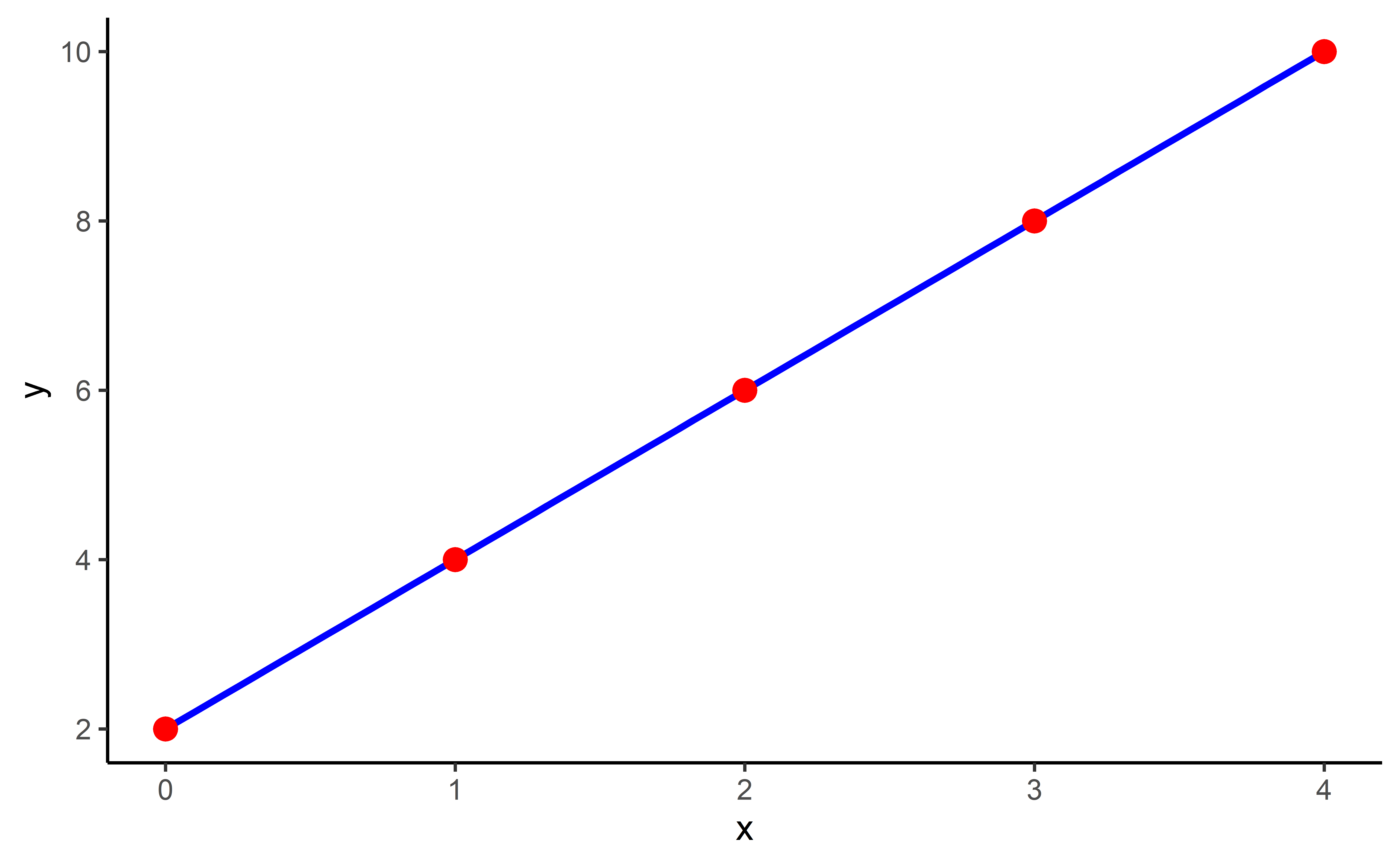
A linha de regressão

\[ y = a + bx \]

y = VI
x = VD
a = constante (local onde a linha intercepta o eixo y, ou seja, onde x = 0)
b = inclinação da linha (cada vez que “x” aumenta 1 unidade, “y” aumenta “b” unidades)

A Linha de Regressão

reg_line

# A tibble: 5 × 2
      x     y
  <dbl> <dbl>
1     0     2
2     1     4
3     2     6
4     3     8
5     4    10

a = 2
b = 2

Regressão Linear Simples

Correlação
- Magnitude e direção
Regressão
- Descobrir o tamanho do efeito de uma variável x (independente, previsora ou explicativa) em uma variável y (dependente, critério ou desfecho)
Questões
- Quanto a pontuação em TMCs pode variar em função da organização do trabalho?
- Quanto a pontuação em TMCs pode variar em função do pertencimento ao grupo de risco para covid-19?

Regressão Linear Simples: Uma Variável Independente Contínua

Quanto a pontuação em TMCs pode variar em função da organização do trabalho?

Análise de Dados Exploratória

Estatística descritiva
- Mínimo
- Máximo
- Média
- Desvio padrão
- Histogramas
Correlações
- Bivariadas
- Gráficos de dispersão

Análise de Dados Exploratória: Uma Olhada nos Dados

Código

df |>
  select(org, tmcs) |> 
  slice_head(n = 10)

# A tibble: 10 × 2
     org  tmcs
   <dbl> <dbl>
 1  1        0
 2  1        2
 3  2.8      1
 4  3        1
 5  2.6      8
 6  3.8     17
 7  3.67    11
 8  2.93     0
 9  2.47     1
10  2.33    20

Análise de Dados Exploratória: Estatísticas Univariadas

Código

df |>
  summarise(
    across(c(tmcs,org),
           list("M" = mean,
                "DP" = sd,
                "MIN" = min,
                "MAX" = max))
    ) |>
  pivot_longer(
    cols = everything(),
    names_to = c("Variável", ".value"),
    names_sep = "_"
    )

# A tibble: 2 × 5
  Variável     M    DP   MIN   MAX
  <chr>    <dbl> <dbl> <dbl> <dbl>
1 tmcs      4.80 4.94      0 20   
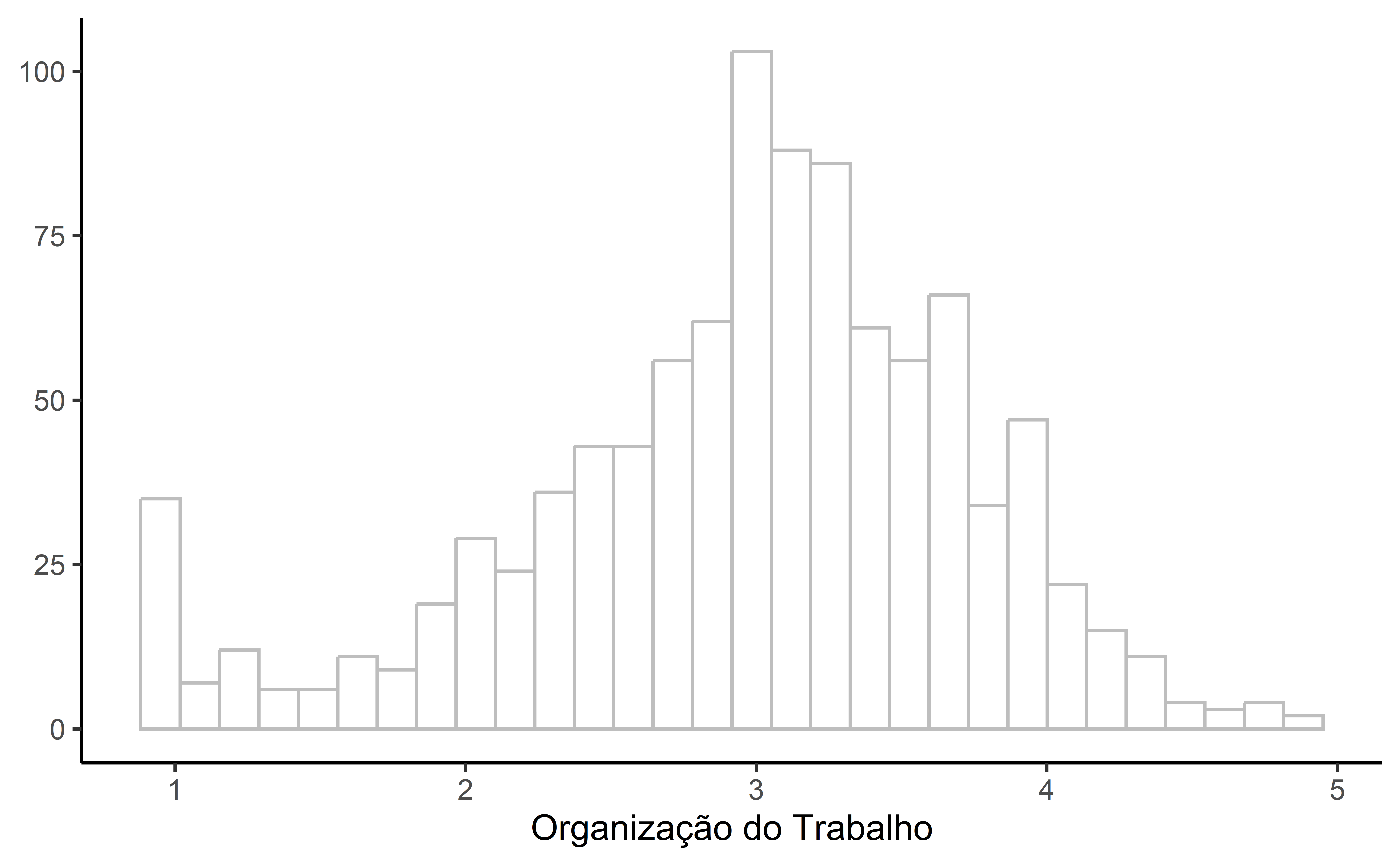
2 org       2.95 0.773     1  4.93

Análise de Dados Exploratória: Estatísticas Univariadas

df |> 
  ggplot(aes(org)) +
  geom_histogram(
    fill = "white",
    color = "gray"
    ) +
  labs(
    y = NULL,
    x = "Organização do Trabalho"
    ) +
  theme_classic()

Análise de Dados Exploratória: Estatísticas Univariadas

Análise de Dados Exploratória: Estatísticas Univariadas

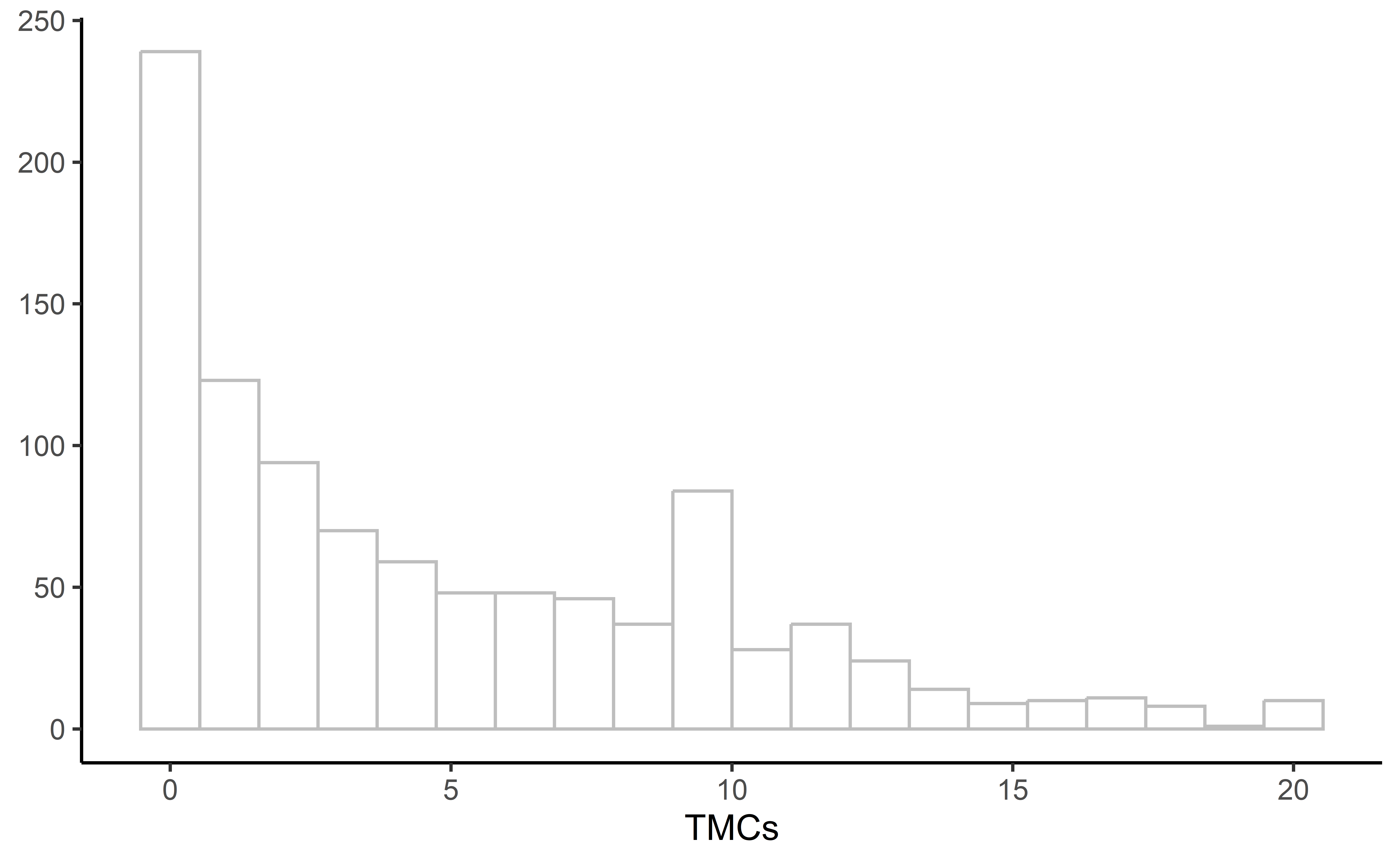
df |> 
  ggplot(aes(tmcs)) +
  geom_histogram(
    fill = "white",
    color = "gray",
    bins = 20
    ) +
  labs(
    y = NULL,
    x = "TMCs"
    ) +
  theme_classic()

Análise de Dados Exploratória: Estatísticas Univariadas

Análise de Dados Exploratória: Estatísticas Bivariadas

2 variáveis numéricas
- Coeficiente de Correlação

Análise de Dados Exploratória: Estatísticas Bivariadas

Código

cor.test(df$org,df$tmcs)


    Pearson's product-moment correlation

data:  df$org and df$tmcs
t = 13.436, df = 998, p-value < 2.2e-16
alternative hypothesis: true correlation is not equal to 0
95 percent confidence interval:
 0.3375806 0.4426364
sample estimates:
     cor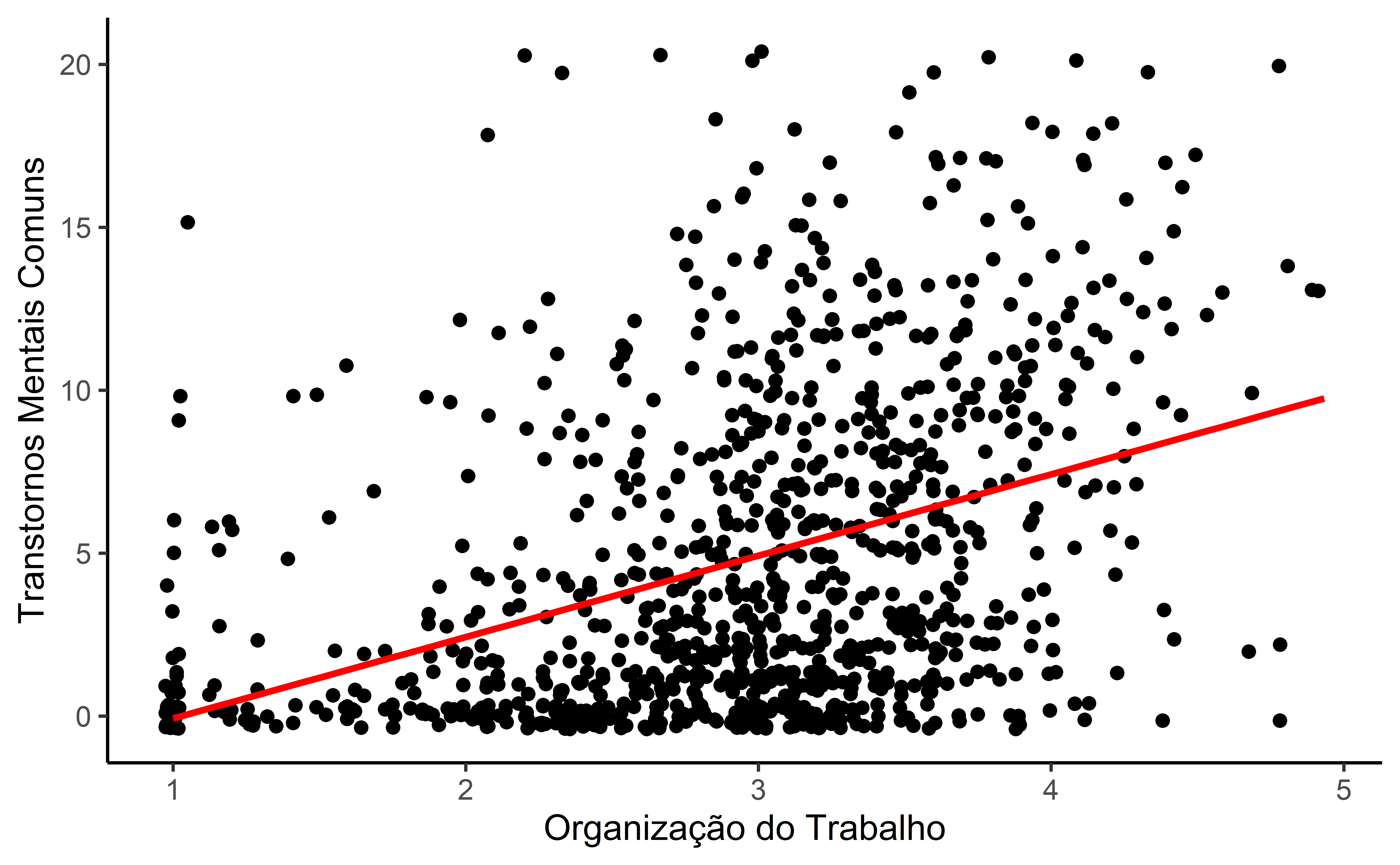 
0.391383

Análise de Dados Exploratória: Estatísticas Bivariadas

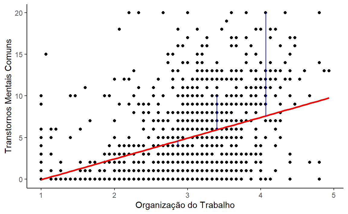
df |> 
  ggplot(aes(org,tmcs)) +
  geom_jitter() +
  geom_smooth(
    method = "lm",
    se = F,
    color = "red"
    ) +
  labs(
    x = "Organização do Trabalho",
    y = "Transtornos Mentais Comuns"
    ) +
  theme_classic()

Análise de Dados Exploratória: Estatísticas Bivariadas

Regressão Linear Simples

\[ y = a + bx \]

A partir do gráfico e do teste de correlação de pearson, o que sabemos até agora sobre entre TMCs e a organização do trabalho? O que podemos dizer sobre a nossa equação?
- b tem uma inclinação positiva!
- Pessoas com piores avaliações da organização do trabalho (escores mais altos) tendem a ter piores índices nos TMCs (pontuações maiores)

Regressão Linear Simples

\[ y = a + bx \]

Qual o valor numérico para a incliação (slope) b?
E o valor do intercepto a?
Vamos utilizar a regressão linear simples para obter essas respostas

Regressão Linear Simples

Notação da regressão:

“~”
VD ~ VI1 + VI2 + VIn

fit_cont <- lm(tmcs ~ org, data = df)

Sumário da saída

Código

summary(fit_cont)


Call:
lm(formula = tmcs ~ org, data = df)

Residuals:
    Min      1Q  Median      3Q     Max 
-9.4166 -3.4224 -0.9221  2.7411 17.0763 

Coefficients:
            Estimate Std. Error t value Pr(>|t|)    
(Intercept)  -2.5703     0.5673  -4.531 6.58e-06 ***
org           2.4973     0.1859  13.436  < 2e-16 ***
---
Signif. codes:  0 '***' 0.001 '**' 0.01 '*' 0.05 '.' 0.1 ' ' 1

Residual standard error: 4.544 on 998 degrees of freedom
Multiple R-squared:  0.1532,    Adjusted R-squared:  0.1523 
F-statistic: 180.5 on 1 and 998 DF,  p-value: < 2.2e-16

Tabela de Regressão

Código

fit_cont |> 
  tidy() |> 
  mutate(
    across(where(is.double),
           \(x) round(x,2))
  )

# A tibble: 2 × 5
  term        estimate std.error statistic p.value
  <chr>          <dbl>     <dbl>     <dbl>   <dbl>
1 (Intercept)    -2.57      0.57     -4.53       0
2 org             2.5       0.19     13.4        0

Tabela de Regressão

tabela_de_regressao <- 
  fit_cont |> 
  tidy() |> 
  mutate(
    across(where(is.double),
           \(x) round(x,2))
    ) |>
  mutate(
    p.value = case_when(p.value == 0 ~ "< .001")
  ) |> 
  rename(
    "Preditor" = term,
    "Estimativas" = estimate,
    "Erro-padrão" = std.error,
    "t" = statistic,
    "p" = p.value
    )

Interpretando a Tabela de Regressão

Código

tabela_de_regressao

# A tibble: 2 × 5
  Preditor    Estimativas `Erro-padrão`     t p     
  <chr>             <dbl>         <dbl> <dbl> <chr> 
1 (Intercept)       -2.57          0.57 -4.53 < .001
2 org                2.5           0.19 13.4  < .001

\[ y = a + bx \]

Estimativas
- a = Estimativa do Intercepto = -2.57
- b = Estimativa da org = 2.50

\[ tmcs = -2.57 + 2.50org \]

Interpretando a Tabela de Regressão

Código

tabela_de_regressao

# A tibble: 2 × 5
  Preditor    Estimativas `Erro-padrão`     t p     
  <chr>             <dbl>         <dbl> <dbl> <chr> 
1 (Intercept)       -2.57          0.57 -4.53 < .001
2 org                2.5           0.19 13.4  < .001

\[ tmcs = -2.57 + 2.50org \]

Quais conclusões podemos tirar dessa equação?
- O sinal de b é positivo, portanto há uma relação positiva entre as variáveis
  - Quanto maior a pontuação em org maior a pontuação em tmcs
  - Ou seja: piores avaliações da organização do trabalho estão associados a maiores prejuízos a saúde mental
- Interpretação do valor de b (estimativa de org):
  - Para cada aumento de 1 unidade em org, há um aumento associado de, em média, 2.50 unidades de tmcs

Interpretando a Tabela de Regressão

Código

cor_org_tmcs <- cor.test(df$org,df$tmcs)

cor_org_tmcs


    Pearson's product-moment correlation

data:  df$org and df$tmcs
t = 13.436, df = 998, p-value < 2.2e-16
alternative hypothesis: true correlation is not equal to 0
95 percent confidence interval:
 0.3375806 0.4426364
sample estimates:
     cor 
0.391383

Código

r <- cor_org_tmcs$estimate

r^2 |> 
  round(4)

   cor 
0.1532

Código

summary(fit_cont)


Call:
lm(formula = tmcs ~ org, data = df)

Residuals:
    Min      1Q  Median      3Q     Max 
-9.4166 -3.4224 -0.9221  2.7411 17.0763 

Coefficients:
            Estimate Std. Error t value Pr(>|t|)    
(Intercept)  -2.5703     0.5673  -4.531 6.58e-06 ***
org           2.4973     0.1859  13.436  < 2e-16 ***
---
Signif. codes:  0 '***' 0.001 '**' 0.01 '*' 0.05 '.' 0.1 ' ' 1

Residual standard error: 4.544 on 998 degrees of freedom
Multiple R-squared:  0.1532,    Adjusted R-squared:  0.1523 
F-statistic: 180.5 on 1 and 998 DF,  p-value: < 2.2e-16

Valores Observados/Ajustados e os Resíduos

\[ tmcs = -2.57 + 2.50org \]

Código

df |>
  mutate(
    id = 1:nrow(df)
  ) |> 
  select(id,tmcs,org) |> 
  slice(15)

# A tibble: 1 × 3
     id  tmcs   org
  <int> <dbl> <dbl>
1    15     4  2.87

Valor observado dos tmcs = 4

\[ tmcs = -2.57 + 2.50*2.867 = 4.598 \]

Valor ajustado/previsto = 4.598
Resíduos: a diferença entre o que foi ajustado/previsto e o valor observado

\[ resíduo = 4 - 4.598 = -0.598 \]

Valores Observados/Ajustados e os Resíduos

df |> 
  ggplot(aes(org,tmcs)) +
  geom_point() +
  geom_smooth(
    method = "lm",
    se = F,
    color = "red"
    ) +
  labs(
    x = "Organização do Trabalho",
    y = "Transtornos Mentais Comuns"
    ) +
  theme_classic()+
  geom_segment(aes(x = 2.867, y = 4, 
                   xend = 2.867, yend = 4.598),
               color = "blue")+
  geom_segment(aes(x = 4.07, y = 20,
                   xend = 4.07, yend = 7.59),
               color = "blue") +
  geom_segment(aes(x = 3.4, y = 10,
                   xend = 3.4, yend = 5.92),
               color = "blue")

Valores Observados/Ajustados e os Resíduos

Valores Observados/Ajustados e os Resíduos

fit_cont |> 
  augment() |> 
  select(tmcs:.resid) |>
  mutate(
    id = 1:nrow(df),
    .before = tmcs
    ) |> 
  slice_head(n = 15) |> 
  mutate(
    across(.fitted:.resid,
           \(x) round(x,3))
    )

Valores Observados/Ajustados e os Resíduos

# A tibble: 15 × 5
      id  tmcs   org .fitted .resid
   <int> <dbl> <dbl>   <dbl>  <dbl>
 1     1     0  1     -0.073  0.073
 2     2     2  1     -0.073  2.07 
 3     3     1  2.8    4.42  -3.42 
 4     4     1  3      4.92  -3.92 
 5     5     8  2.6    3.92   4.08 
 6     6    17  3.8    6.92  10.1  
 7     7    11  3.67   6.59   4.41 
 8     8     0  2.93   4.76  -4.76 
 9     9     1  2.47   3.59  -2.59 
10    10    20  2.33   3.26  16.7  
11    11    12  3.67   6.59   5.41 
12    12     0  2.73   4.26  -4.26 
13    13     2  3.13   5.26  -3.26 
14    14     3  3.67   6.59  -3.59 
15    15     4  2.87   4.59  -0.589

Regressão Linear Simples: Uma Variável Independente Categórica

Quanto a pontuação em TMCs pode variar em função do pertencimento ao grupo de risco para covid-19?

Análise de Dados Exploratória

Estatística descritiva
- Variável Dependente (contínua)
  - Mínimo
  - Máximo
  - Média
  - Desvio padrão
- Variável independente (categórica)
  - Tabela de frequência
- Gráficos para comparação entre médias/medianas
  - Boxplot
- Tabelas para compração entre grupos
- Teste T para amostras independentes (VI dicotômica)

Análise de Dados Exploratória: Uma Olhada nos Dados

Código

df |> 
  select(tmcs, grupo_de_risco) |> 
  slice_head(n = 10)

# A tibble: 10 × 2
    tmcs grupo_de_risco
   <dbl> <chr>         
 1     0 Não           
 2     2 Sim           
 3     1 Não           
 4     1 Sim           
 5     8 Não           
 6    17 Não           
 7    11 Não           
 8     0 Sim           
 9     1 Não           
10    20 Não

Análise de Dados Exploratória: Estatísticas Univariadas

Código

df |>
  summarise(
    across(c(tmcs),
           list("M" = mean,
                "DP" = sd,
                "MIN" = min,
                "MAX" = max))
    ) |>
  pivot_longer(
    cols = everything(),
    names_to = c("Variável", ".value"),
    names_sep = "_"
    )

# A tibble: 1 × 5
  Variável     M    DP   MIN   MAX
  <chr>    <dbl> <dbl> <dbl> <dbl>
1 tmcs      4.80  4.94     0    20

Análise de Dados Exploratória: Estatísticas Univariadas

df |> 
  ggplot(aes(tmcs)) +
  geom_histogram(
    fill = "white",
    color = "gray",
    bins = 20
    ) +
  labs(
    y = NULL,
    x = "TMCs"
    ) +
  theme_classic()

Análise de Dados Exploratória: Estatísticas Univariadas

Análise de Dados Exploratória: Tabelas de Frequência

Código

df |> 
  count(grupo_de_risco) |> 
  mutate(
    "%"   = (n/sum(n))*100
         )

# A tibble: 2 × 3
  grupo_de_risco     n   `%`
  <chr>          <int> <dbl>
1 Não              754  75.4
2 Sim              246  24.6

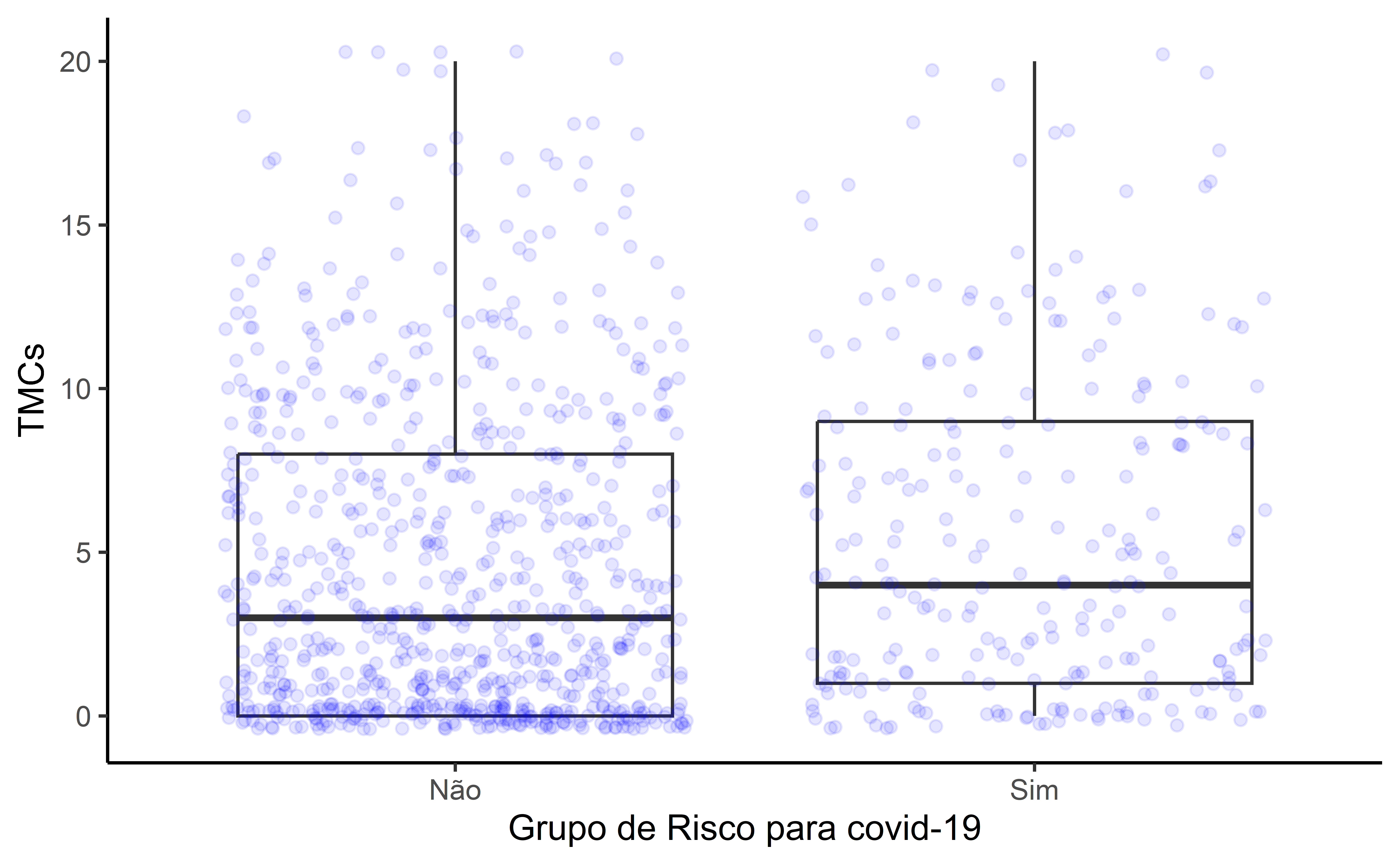
Comparação entre Grupos

df |> 
  ggplot(aes(grupo_de_risco,tmcs))+
  geom_boxplot() +
  geom_jitter(aes(grupo_de_risco),
              alpha = 0.1,
              size = 1.5,
              color = "blue") +
  labs(
    x = "Grupo de Risco para covid-19",
    y = "TMCs"
    ) +
  theme_classic()

Comparação entre Grupos

Resultados entre Grupos

Código

df |> 
  group_by(grupo_de_risco) |> 
  summarise(
    M = mean(tmcs),
    DP = sd(tmcs),
    MD = median(tmcs),
    MIN = min(tmcs),
    MAX = max(tmcs)
    )

# A tibble: 2 × 6
  grupo_de_risco     M    DP    MD   MIN   MAX
  <chr>          <dbl> <dbl> <dbl> <dbl> <dbl>
1 Não             4.53  4.83     3     0    20
2 Sim             5.63  5.18     4     0    20

Diferenças Entre as Médias

Código

medias <- df |> 
  group_by(grupo_de_risco) |> 
  summarise(
    M = mean(tmcs)
    )

dif <- medias |>
  mutate(
    DIF = M - (medias |> 
                 filter(grupo_de_risco == "Não") |> 
                 select(M) |> 
                 unlist(use.names = F))
)

dif

# A tibble: 2 × 3
  grupo_de_risco     M   DIF
  <chr>          <dbl> <dbl>
1 Não             4.53  0   
2 Sim             5.63  1.10

Diferenças Entre as Médias

Código

t.test(tmcs ~ fct_relevel(grupo_de_risco, "Sim"), data = df,var.equal = T)


    Two Sample t-test

data:  tmcs by fct_relevel(grupo_de_risco, "Sim")
t = 3.0395, df = 998, p-value = 0.002431
alternative hypothesis: true difference in means between group Sim and group Não is not equal to 0
95 percent confidence interval:
 0.3887405 1.8051091
sample estimates:
mean in group Sim mean in group Não 
         5.630081          4.533156

Regressão Linear Simples

fit_cat <- lm(tmcs ~ grupo_de_risco, data = df)

Sumário da Regressão

Código

summary(fit_cat)


Call:
lm(formula = tmcs ~ grupo_de_risco, data = df)

Residuals:
   Min     1Q Median     3Q    Max 
-5.630 -4.533 -1.533  3.370 15.467 

Coefficients:
                  Estimate Std. Error t value Pr(>|t|)    
(Intercept)         4.5332     0.1790   25.33  < 2e-16 ***
grupo_de_riscoSim   1.0969     0.3609    3.04  0.00243 ** 
---
Signif. codes:  0 '***' 0.001 '**' 0.01 '*' 0.05 '.' 0.1 ' ' 1

Residual standard error: 4.915 on 998 degrees of freedom
Multiple R-squared:  0.009172,  Adjusted R-squared:  0.00818 
F-statistic: 9.239 on 1 and 998 DF,  p-value: 0.002431

Tabela de Regressão

Código

tabela_de_regressao_cat <- 
  fit_cat |>
  tidy() |> 
  mutate(
    across(where(is.double),
                \(x) round(x,2))
    ) |>
  mutate(
    p.value = case_when(p.value == 0 ~ "< .001")
  ) |> 
  rename(
    "Preditor" = term,
    "Estimativas" = estimate,
    "Erro-padrão" = std.error,
    "t" = statistic,
    "p" = p.value
    )

Interpretando a Tabela de Regressão

Código

tabela_de_regressao_cat

# A tibble: 2 × 5
  Preditor          Estimativas `Erro-padrão`     t p     
  <chr>                   <dbl>         <dbl> <dbl> <chr> 
1 (Intercept)              4.53          0.18 25.3  < .001
2 grupo_de_riscoSim        1.1           0.36  3.04 < .001

Estimativa do Intercepto = média do grupo_de_riscoNão = 4.53
Estimativa do grupo_de_riscoSim = diferença entre a média do grupo_de_riscoNao e a média grupo_de_riscoSim = 1.10

Código

dif

# A tibble: 2 × 3
  grupo_de_risco     M   DIF
  <chr>          <dbl> <dbl>
1 Não             4.53  0   
2 Sim             5.63  1.10